Module Documentation

C-LAB 26.08.0 · October 2026

1About#

This document describes the API of the C-LAB Python module distributed with C-LAB 26.08.0. Get the latest version from https://www.c-lab.tech.

For additional information, support, or feedback, contact us at info@c-lab.tech.

Python® is a registered trademark of the Python Software Foundation.

2Classes#

C-LAB module defines 6 custom classes, as listed below. Refer to each section for further information.

clab.Array: Stores data as a contiguous array of IEEE 754 double-precision (64-bit) floating-point values.
clab.Container: Container with all variables (as TimeSeries) read from file.
clab.Mesh: Stores mesh data to be used in surface 3D plots.
clab.Model: Simulation model object.
clab.Result: Container with data results from a simulation model.
clab.TimeSeries: Stores series of data indexed in chronological order.

2.1clab.Array#

clab.Array stores data as a contiguous array of IEEE 754 double-precision (64-bit) floating-point values.

Constructor

An instance of clab.Array can be created directly using the following functions:

clab.Array(list)

listrequired: Python list with numeric values. Behavior with non-numeric types is undefined.

clab.Array(other)

otherrequired: clab.Array. This constructor will shallow-copy other to the new object. Therefore, both objects will share the same underlying data values: modifications done in one object will reflect upon the other. Check the clone function if a deep-copy is required.

clab.Array(len)

lenrequired: Length of the new array. The new clab.Array will be zero-initialized.

Member Variables

clab.Array has no publicly exposed member variables.

Member Functions

clab.Array implements the Number Protocol, supporting standard arithmetic operations: addition, subtraction, multiplication, remainder, division, exponentiation, bitwise AND ( $\mathtt{\&}$ ), bitwise XOR (^), bitwise OR ( $\mathtt{|}$ ), negation ( $\mathtt{\sim}$ ), and absolute value. In-place equivalents are also supported.

clab.Array implements the Sequence Protocol, allowing element access via the standard $\texttt{[]}$ operator.

Besides standard protocols, the following member functions are available:

out = clab.Array.clone()

out: clab.Array.

Return a new clab.Array containing a deep-copy of the caller’s values.

out = clab.Array.to_list()

out: Python list with the same length as the clab.Array.

Export array values as a standard Python list.

out = clab.Array.avg()

out: Float.

Return the arithmetic mean (average) of the array’s values.

out = clab.Array.sum()

out: Float.

Return the sum of all elements in the array.

out = clab.Array.count_eq(val)

out: Integer.
valrequired: Numeric value.

Return the number of elements in the array that are exactly equal to val.

out = clab.Array.count_gt(val)

out: Integer.
valrequired: Numeric value.

Return the count of elements that are strictly greater than val.

out = clab.Array.count_lt(val)

out: Integer.
valrequired: Numeric value.

Return the count of elements that are strictly less than val.

out = clab.Array.count_bt(val1, val2)

out: Integer.
val1required: Numeric lower bound.
val2required: Numeric upper bound.

Return the count of elements that are strictly between the provided arguments, i.e., $> \texttt{val1}$ and $< \texttt{val2}$ .

out = clab.Array.logical_and(rhs)

out: clab.Array.
rhs: clab.Array.

Return a new array (containing 0s and 1s) resulting from the logical AND operation between the current array and clab.Array rhs.

out = clab.Array.logical_or(rhs)

out: clab.Array.
rhs: clab.Array.

Return a new array (containing 0s and 1s) resulting from the logical OR operation between the current array and clab.Array rhs.

out = clab.Array.logical_not()

out: clab.Array.

Return a new array (containing 0s and 1s) representing the logical NOT operation on all elements.

out = clab.Array.logical_xor(rhs)

out: clab.Array.
rhs: clab.Array.

Return a new array (containing 0s and 1s) resulting from the logical XOR operation between the current array and clab.Array rhs.

2.2clab.Container#

The clab.Container class stores variables loaded from a file or acquired from a real-time source (experimental feature). Each clab.TimeSeries is also exposed as an attribute of the container, with its name automatically converted into a valid Python identifier.

Constructor

An instance of clab.Container can be created using:

clab.Container(path, plugin='', realtime=False, samples=300)

pathrequired

Full path to the input file.

If the file is compressed, C-LAB will first decompress it into the cache directory and then load the extracted file using the appropriate loader.

pluginoptional

Full path to a plugin.

If omitted, C-LAB automatically selects a compatible loader by testing installed plugins and built-in loaders. If provided, the specified plugin is used directly, bypassing compatibility checks.

realtimeoptional

[experimental] Enables acquisition from a real-time data source when set to True.

This feature is experimental and its API may change in future releases.

samplesoptional

[experimental] Maximum number of samples stored when acquiring real-time data.

Once this limit is reached, older samples are discarded to accommodate new data. This feature is experimental and subject to change.

Member Variables

clab.Container.id64integer

Read-only. Unique 64-bit identifier.

clab.Container.flagsinteger

Read-only. Reserved for internal use.

Member Functions

clab.Container partially implements the Mapping Protocol, allowing access to individual clab.TimeSeries objects via the [] operator using their source names.

In addition to standard protocol behavior, the following member functions are available:

out = clab.Container.get_path()

out: List.

Returns the list of file paths associated with the container.

out = clab.Container.get_size()

out: Integer.

Returns the number of TimeSeries objects in the container.

clab.Container.axpb(a, b)

arequired: Numeric value.
brequired: Numeric value.

Applies the transformation $A \cdot X + B$ to the x-axis of all variables.

If the data is not yet loaded, the operation is deferred until loading completes.

clab.Container.aypb(a, b)

arequired: Numeric value.
brequired: Numeric value.

Applies the transformation $A \cdot Y + B$ to the y-axis of all variables.

If the data is not yet loaded, the operation is deferred until loading completes.

clab.Container.merge(path)

pathrequired: File path.

Merges the contents of the specified file into the container.

All TimeSeries loaded after this call will use data from this file in addition to previously loaded sources. Already loaded TimeSeries remain unchanged.

clab.Container.replace_xdata(ts)

tsrequired: clab.TimeSeries used as the source for x-axis data.

Replaces the x-axis data of all contained variables using the y-data from ts.

The source data must be strictly increasing (monotonically increasing with no repeated or decreasing values).

If data sizes differ, the maximum compatible subset is copied without overflow, and a warning message is issued.

clab.Container.rt_read()

Refreshes data from a real-time source by invoking the Load function (see Section 5.1.2).

clab.Container.rt_start()

Starts real-time data acquisition by invoking the Start function (see Section 5.1.2).

clab.Container.rt_stop()

Stops real-time data acquisition by invoking the Stop function (see Section 5.1.2).

2.3clab.Mesh#

clab.Mesh stores clab.Array data of the x, y and z-axis to be plotted in a surface mesh plot. X and Z are the input of the mesh function. Y is the output matrix, where x values are stored contiguously:

$Y = \left( \begin{matrix} y_{x:0,z:0} & y_{x:1,z:0} & y_{x:2,z:0} & \cdots \\ y_{x:0,z:1} & y_{x:1,z:1} & y_{x:2,z:1} & \cdots \\ \vdots & \vdots & \vdots & \\ y_{x:0,z:N} & y_{x:1,z:N} & y_{x:2,z:N} & \cdots \end{matrix} \right)$

Constructor

An instance of clab.Mesh can be created directly using the following functions:

clab.Mesh()

Create an empty clab.Mesh object.

Member Variables

clab.Mesh.id64integer

Read-only. Unique 64-bit identifier assigned upon creation.

clab.Mesh.flagsinteger

Read-only. Internal use only.

clab.Mesh.xdataclab.Array

clab.Array containing the data points for the x-axis coordinates.

clab.Mesh.ydataclab.Array

clab.Array containing the data values for the y-coordinate, corresponding to the specified $x$ and $z$ pairs.

clab.Mesh.zdataclab.Array

clab.Array containing the data points for the z-axis coordinates.

Member Functions

clab.Mesh has no public member functions.

2.4clab.Model#

The clab.Model class represents a simulation model. It can be created programmatically or loaded from a JSON file and used for validation, execution, and code generation.

Constructor

An instance of clab.Model can be created using:

clab.Model()

Creates an empty clab.Model.

clab.Model(path)

path: String with the full path to a JSON file.

Creates a clab.Model by loading the JSON file located at the given path.

Member Variables

clab.Model.flagsinteger

Read-only. Internal use only.

Member Functions

out = clab.Model.get(key, id)

out

Value of the requested parameter.

keyrequired

String with the parameter name. It can be one of the following values:

inportCount: Number of inports.
outportCount: Number of outports.
x: Block position (x-axis).
y: Block position (y-axis).
width: Block dimension.
height: Block dimension.
red: Block color channel.
green: Block color channel.
blue: Block color channel.
ti: Simulation initial time (seconds).
tf: Simulation final time (seconds).
ts: Simulation step time (seconds).

idoptional

Block unique identifier. Required when accessing block-specific parameters.

Returns model-level or block-level parameters.

Examples

model.get(key='ts')
model.get(key='x', id=1234)

clab.Model.set(...)

idoptional: Block unique identifier. Required when modifying block parameters.
xoptional: Block position (x-axis).
yoptional: Block position (y-axis).
widthoptional: Block dimension.
heightoptional: Block dimension.
redoptional: Block color channel. Values outside the range [0.0, 1.0] are ignored.
greenoptional: Block color channel. Values outside the range [0.0, 1.0] are ignored.
blueoptional: Block color channel. Values outside the range [0.0, 1.0] are ignored.
tioptional: Simulation initial time (seconds).
tfoptional: Simulation final time (seconds).
tsoptional: Simulation step time (seconds).

Sets model-level or block-level parameters.

Examples

model.set(ti=5.0, tf=10.0)
model.set(id=1234, x=10, y=20)

out = clab.Model.create(class, ...)

out

Block unique identifier.

classrequired

Block class. It can be one of the following values:

abs: Calculates the absolute value of the input.
acc: Outputs the sum of values from the first port; resets the accumulation to the value of the second port if the third port is True.
acos: Calculates the arccosine of the input.
add: Computes the sum of all inputs.
asin: Calculates the arcsine of the input.
atan: Calculates the arctangent of the input.
cast: Converts the input to a different data type, as specified by the type parameter ('bool', 'int8', 'int16', 'int32', 'int64', 'uint8', 'uint16', 'uint32', 'uint64', 'flt32', 'flt64').
clamp: Limits the value of the first input based on the boundaries set by the second and third inputs.

constant: Represents a constant value source, with its value defined by the expression parameter.
cos: Calculates the cosine of the input.
debounce: Debounces input signals, introducing a delay to filter out rapid changes or noise.
delta: Computes the difference between the current sample and the previous one.
display: Displays input data.
divide: Computes the quotient of the first input divided by the second input.
enable: Enables or disables sub-system simulation. By default, enable ports are assigned to the port number -1.
from: Used with goto as an alternative for line connections. This block connects to its goto counterpart by its target parameter.
from_workspace: Imports data from a clab.TimeSeries variable, set by the obj parameter.
goto: Used with from as an alternative for line connections. This block connects to its from counterpart by its target parameter.
hysteresis: The output is True when the input is greater than valueOn and False when it is less than valueOff. Otherwise, it keeps its last value.
if: Implements conditional logic.
inport: Represents an input port for receiving external signals into a subsystem. Its number is set by the portNumber parameter (zero-based indexing).
lerp: Computes linear interpolation between two values. Effectively, it outputs $A + U\times (B - A)$ . The equation coefficients are set by the coeffA and coeffB parameters.
log: Computes the logarithm (base $e$ ) of the input.
logical: Performs logical operations on input signals. The logical operation is set by the operator parameter ('and', 'or', 'nand', 'nor').
lut1d: Performs a one-dimensional lookup table operation. Its values are set by the out and out parameters.
lut2d: Performs a two-dimensional lookup table operation. Its values are set by the out, bp1 and bp2 parameters.
max: Determines the maximum value among all input samples.
memory: Delays input sample, by storing its current value and outputting it on the next simulation loop.
min: Determines the minimum value among all input samples.
mod: Calculates the remainder of the division of the first input by the second input.
multiply: Computes the multiplication of all input values.
not: Performs logical negation, converting True to False and vice versa.
outport: Represents an output port for transmitting signals out of the subsystem. Its number is set by the portNumber parameter (zero-based indexing).
poly1st: Outputs the result of a first-order polynomial, as $f(x) = A \times x + B$ . The equation coefficients are set by the coeffA and coeffB parameters.
pow: Raises the first input to the power of the second input.
ramp: Generates a ramp, defined by the initialValue, finalValue and time parameters.
random: Generates random values, defined by the min, max and seed parameters.
refsys: Represents a reference to a subsystem defined in an external file, set by the path parameter.

relational: Compares input values based on relational operations, set by the operator parameter ('eq', 'ge', 'gt', 'le', 'lt', 'ne').
sin: Calculates the sine of the input.
sinewave: Generates a sinusoidal waveform, as specified by the frequency and phase parameters. The frequency is given in hertz and the phase, in degrees.
sqrt: Calculates the square root of the input.
squarewave: Generates a square waveform, as specified by the timeOn, timeOff, valueOn and valueOff parameters.
step: Outputs a step function, defined by the initialValue, finalValue and time parameters.
subsys: Represents a subsystem or a modular block that encapsulates a specific functionality within a larger system.
subtract: Calculates the difference between the first input and the second input.
switch: Routes input signals to the output based on a control signal.
tan: Calculates the tangent of the input.
time: Outputs the current simulation time.
to_workspace: Exports to a clab.TimeSeries variable, whose name is set by the name parameter.
unpack: Unpacks the input value, selecting the desired bits and applying gain and bias (bit extraction), as specified by the lsb, msb, coeffA and coeffB parameters. The bits indexing is zero-based.

nameoptional

Block name.

parentoptional

Parent block identifier. If omitted, the block is created in the root subsystem.

Creates a new block and returns its unique identifier.

Examples

model = clab.Model()
c0 = model.create('constant', expression=3.14)
s0 = model.create('sinewave', frequency=2.0)

clab.Model.link(blockFrom, blockTo, portFrom, portTo, name)

blockFromrequired: Source block identifier.
blockTorequired: Destination block identifier.
portFromrequired: Source port index (zero-based).
portTorequired: Destination port index (zero-based).
nameoptional: Connection label.

Creates a connection between blocks.

Examples

model.link(blockFrom=b1, blockTo=b2, portFrom=0, portTo=1)

clab.Model.codegen(lang, path)

langrequired: Target language: 'c' or 'python'.
pathrequired: Output directory path.

Generates source code from the model. Raises an exception on failure.

out = clab.Model.load(path)

out: Error code.
pathrequired: JSON file path.

Loads a model from disk.

clab.Model.run()

Runs the simulation. Raises an exception on failure.

clab.Model.validate()

Validates the model. Raises an exception if errors are found.

2.5clab.Result#

The clab.Result class stores the output data generated by a simulation. Each subsystem in the model is represented by a corresponding clab.Result object.

Constructor

An instance of clab.Result can be created using:

clab.Result()

Creates an empty clab.Result.

Member Variables

clab.Result.flagsinteger

Read-only. Internal use only.

Member Functions

clab.Result does not provide any member functions.

2.6clab.TimeSeries#

clab.TimeSeries stores two clab.Array instances of the same size, holding the x-axis data (typically time, hence the name TimeSeries) and the y-axis data. The x-axis values are expected to be strictly increasing, i.e., $xdata_{k} < xdata_{k+1}$ for any given $k$ .

Constructor

An instance of clab.TimeSeries can be created directly using the following functions:

clab.TimeSeries()

Create an empty clab.TimeSeries object. It’s recommended not to use this function. It’s listed here only for the sake of completeness.

clab.TimeSeries(id64)

id64required: Unique identifier.

Create a clab.TimeSeries from a valid variable identifier id64. This is for internal usage only.

clab.TimeSeries(xvalues, yvalues)

xvaluesrequired: Python List or Python Tuple with the x-axis values. All elements in the sequence must be numeric.
yvaluesrequired: Python List or Python Tuple with the y-axis values. All elements in the sequence must be numeric.

Create a clab.TimeSeries from two Python Lists or from two Python Tuples. The first one has the values for the x-axis and the second one for the y-axis.

clab.TimeSeries(rhs)

rhsrequired: clab.TimeSeries.

Create a clab.TimeSeries from another clab.TimeSeries rhs. Both objects will share the same xdata and ydata objects (shallow copy).

Member Variables

clab.TimeSeries.id64integer

Read-only. Unique 64-bit identifier.

clab.TimeSeries.flagsinteger

Read-only. Internal use only.

clab.TimeSeries.xdataclab.Array

Read/write. clab.Array object that stores data to be used in the x-axis (typically time in seconds).

clab.TimeSeries.ydataclab.Array

Read/write. clab.Array object that stores data to be used in the y-axis.

Member Functions

clab.TimeSeries implements the Number Protocol, i.e., clab.TimeSeries supports the standard operations: add, subtract, multiply, remainder, divide, power, and (&), xor (^), or (|) (and their in-place equivalents), negative ( $\mathtt{\sim}$ ), absolute. For all the aforementioned functions that require two or more operands, the ydata is aligned over time using the xdata values.

clab.TimeSeries partially implements the Mapping Protocol, meaning that it’s possible to access each clab.TimeSeries in the container using the [] operator providing the child’s source name.

clab.TimeSeries implements the Sequence Protocol, meaning that it’s possible to read each x-y pair in the TimeSeries using the [] operator. Each item contains a two-element tuple: the first element contains the x value and the second, the y value.

Besides the standard protocols, the following member functions are available:

out = clab.TimeSeries.get_name()

out: String.

Return variable’s name. Only available for data loaded directly from sources; calculated variables return an empty string.

out = clab.TimeSeries.get_fs()

out: Sampling frequency in hertz.

Return the estimated sampling frequency in hertz. If the object has not been loaded yet, this function will force it.

out = clab.TimeSeries.get_ts()

out: Sampling period in seconds.

Return the estimated sampling period in seconds. If the object has not been loaded yet, this function will force it.

out = clab.TimeSeries.axpb(a, b)

arequired: Numeric value.
brequired: Numeric value.

Apply $A \cdot X+B$ for all values in the x-axis. If the data is empty, this operation will be postponed until the data has been successfully loaded.

out = clab.TimeSeries.aypb(a, b)

arequired: Numeric value.
brequired: Numeric value.

Apply $A \cdot Y+B$ for all values in the y-axis. If the data is empty, this operation will be postponed until the data has been successfully loaded.

out = clab.TimeSeries.avg()

out: Float value.

Return the average of the object’s yvalues.

out = clab.TimeSeries.max()

out: Float value.

Return the maximum of the object’s yvalues.

out = clab.TimeSeries.min()

out: Float value.

Return the minimum of the object’s yvalues.

out = clab.TimeSeries.sum()

out: Float value.

Return the sum of the object’s yvalues.

out = clab.TimeSeries.index(val, op='eq')

out: Integer value.
valrequired: Numeric value.
opoptional: Operator used by search. Valid operators are eq, ne, le, lt, ge or gt.

Return sample index that match the search criteria.

clab.TimeSeries.inspect()

Print TimeSeries internal information for debugging and troubleshooting.

clab.TimeSeries.load()

Load TimeSeries values from source file, if they haven’t been already. On success, the members xdata and ydata are filled with the loaded values.

out = clab.TimeSeries.slice(tini, tend)

out: clab.TimeSeries.
tinirequired: Numeric value. Slice initial time.
tendrequired: Numeric value. Slice final time.

Return a new object containing a slice (or subsequence) of the source object, within the limits defined by the arguments.

clab.TimeSeries.sort()

Sort samples chronologically (i.e. by x-axis values).

out = clab.TimeSeries.tag(val)

out: String value.
valrequired: Numeric value.

Return the tag associated with the value val for this object. If there’s no tag associated, it will return 'n/a'.

out = clab.TimeSeries.time_eq(val)

out: Numeric value.
valrequired: Numeric value.

Return total time in which y-axis values are equal to val.

out = clab.TimeSeries.time_ne(val)

out: Numeric value.
valrequired: Numeric value.

Return total time in which y-axis values are not equal to val.

out = clab.TimeSeries.time_gt(val)

out: Numeric value.
valrequired: Numeric value.

Return total time in which y-axis values are greater than val.

out = clab.TimeSeries.time_lt(val)

out: Numeric value.
valrequired: Numeric value.

Return total time in which y-axis values are less than val.

out = clab.TimeSeries.time_bt(val1, val2)

out: Numeric value.
val1required: Numeric lower bound.
val2required: Numeric upper bound.

Return total time in which y-axis values are between the provided arguments, i.e., simultaneously greater than val1 and less than val2.

3Settings#

Settings can be configured through the dedicated tab in the application UI or via the module functions (see Section 3.3).

3.1UI Settings#

3.1.1UI Theme#

Controls the color theme of the user interface. Default: 'dark'.

Setting this option to 'lite' enables the lite theme.

Changes are applied immediately.

3.1.2Export Theme#

Controls the color theme used when exporting charts to files. Default: 'dark'.

Setting this option to 'lite' enables the lite theme for exported charts. This allows dark UI users to export charts with a light background without changing the UI theme.

Changes are applied immediately.

3.2General Settings#

3.2.1Autosave#

Enables autosave and defines the interval for saving charts and models in memory to a backup file.

Autosave files are stored in: C:\Users\<user>\.clab\cache.

3.2.2Log Severity Level#

Defines the minimum severity level to be logged. Supported values (in increasing order): Trace, Debug, Info, Warning, Error, Fatal.

Logs are stored in: C:\Users\<user>\.clab\logs.

Restart required.

3.2.3Tags File Path#

Path to a TSV file used to assign tags to specific values in data tips.

If both the parameter name and value match an entry, the corresponding tag is displayed.

Useful for parameters with discrete meanings (e.g., states, modes).

An example file is available in the example directory of the installation folder.

Required TSV columns:

Source: Parameter name.
Value: Parameter value.
Tag: Displayed text.

Restart not required.

3.2.4Unpack File Path#

Path to a TSV file used to automatically unpack clab.TimeSeries data. If a parameter name matches an entry, its data is unpacked into one or more derived series, equivalent to clab.unpack() (see Section 6.2.8).

An example file is available in the example directory of the installation folder.

Required TSV columns:

Source: Parameter name used for matching.
Alias: Name of the generated series.
MSB: Most significant bit (see Indexing).
LSB: Least significant bit (see Indexing).
Resolution: Scaling factor in the transformation.
Offset: Offset in the transformation.
Unit: Documentation only.
Type: Conversion type: 2C, BCD, or BNR.
Indexing: Bit indexing scheme (e.g., 0 for zero-based).

Transformation: alias = source[msb:lsb] $\times$ resolution $+$ offset

Restart not required.

3.2.5Python Dynamic Library Path#

Specifies the path to the Python 3 dynamic library (.dll) used by C-LAB.

If not set, the embedded version is used: C:\<clab folder>\python\python3.dll.

Restart required.

3.2.6Memory Allowed#

Defines the maximum fraction of system RAM that C-LAB may use. Default: 80%.

If the limit is exceeded, least frequently used data is unloaded until usage falls below the threshold.

Memory usage (used, available, total) is displayed in the application status area.

Restart required.

3.3Using the Module#

3.3.1Read Configuration Values#

out = clab.get_config(key, group)

out: Value associated with the specified key.
keyrequired: Setting key.
groupoptional: Setting group. Default: 'general'.

Examples

value = clab.get_config(key='memory')

3.3.2Write Configuration Values#

Some changes are applied only after the module is reloaded, as with updates made through the UI. See Sections Section 3.1 and Section 3.2 for details.

clab.set_config(key, group, value)

keyrequired

Setting key. Supported values:

file: Export theme. Values: 'dark', 'lite'. Group: 'theme'.
ui: UI theme. Values: 'dark', 'lite'. Group: 'theme'.
x: Window horizontal position. Group: 'window'.
y: Window vertical position. Group: 'window'.
height: Window height. Group: 'window'.
width: Window width. Group: 'window'.

groupoptional

Setting group. Default: 'general'.

valuerequired

Setting value.

Examples

clab.set_config(key='memory', value='80')
clab.set_config(key='ui', group='theme', value='dark')
clab.set_config(key='width', group='window', value=800)

3.3.3Reload Configuration Values from File#

Reloads configuration data from file. Required only if the configuration file is modified externally.

clab.reload_config()

4Loading Data From Files#

C-LAB supports loading data from a wide range of file formats using either native loaders or external plugins.

C-LAB does not require the user to explicitly specify the file format. Instead, format detection is performed automatically.

Format Resolution#

When a file is opened, C-LAB determines the appropriate loader using the following procedure:

C-LAB queries all available plugins to determine compatibility with the target file. Each plugin MUST evaluate the file and indicate whether it can handle the format.
If no plugin reports compatibility, C-LAB attempts to load the file using its native loaders.

Compressed Files#

If the input file is a compressed archive, C-LAB will extract its contents to a cache directory prior to loading.

After extraction, C-LAB applies the standard format resolution process to the extracted file(s).

4.1Built-In Loaders#

4.1.1ArduPilot Dataflash Logs#

File Extensions: *.bin, *.log
Supported Data Types: Numeric and string values only.
Reference: https://ardupilot.org/copter/docs/common-downloading-and-analyzing-data-logs-in-mission-planner.html

4.1.2Delimiter-Separated Values#

File Extensions: *.csv, *.tsv, *.txt
Format: Values will be separated by a delimiter character.
Supported Delimiters: comma (ASCII 0x2C), semicolon (ASCII 0x3B), pipe (ASCII 0x7C), tab (ASCII 0x09).
Header: The first row will contain parameter names.
Time Axis: The first column will contain time values.

4.1.3Hierarchical Data Format (HDF5)#

File Extensions: *.hdf5, *.h5
Supported Numeric Types: One-dimensional arrays of signed/unsigned integers (8, 16, 32, 64-bit) and IEEE 754 single/double precision.
Supported String Types: Two-dimensional arrays of fixed-length or variable-length ASCII strings.
String Handling: String values will be mapped to unique numeric identifiers.
Time Axis: Array indices will be used as x-axis values.

4.1.4IRIG106 Chapter 10 Files#

File Extensions: *.ch10
Status: Experimental. This feature may be subject to change in future releases.
Formats: A429, Analog, Video (Only Transport Streams).

4.1.5Microsoft Excel (2007–2013)#

File Extensions: *.xlsx
Header: The first row will contain parameter names.
Time Axis: The first column will contain time values.
Limitations: Formulas are not supported; only evaluated values may be processed.

4.1.6MATLAB/Octave MAT Files#

File Extensions: *.mat
Supported Numeric Types: Arrays of signed/unsigned integers (8, 16, 32, 64-bit) and IEEE 754 single/double precision.
Time Axis: Array indices will be used as x-axis values.
Limitations: Cells, structures, and non-numeric objects are not supported.
Supported Versions: Versions 4, 5, and 7.3.

4.1.7Network Common Data Form (NetCDF) Files#

File Extensions: *.nc
Status: Experimental. This feature may be subject to change in future releases.

4.1.8Parquet Files#

File Extensions

*.parquet, *.gzip

Data Mapping

Each column will be treated as an independent variable.

Supported Types

Only numeric columns are processed; non-numeric columns are ignored.

Null Handling

Null samples will be skipped.

Time Axis

If one or more time-typed columns are present, the first (lowest index) will be used as the time vector.

If no time-typed column is present, the time vector will be generated as a strictly increasing sequence starting at zero.

4.1.9Waveform Audio File Format (WAV)#

File Extensions: *.wav
Description: Standard uncompressed audio file format.

4.2Custom DLL Plugin Loaders#

C-LAB supports custom Dynamic Link Libraries (DLLs) as user-defined plugins for loading data from files.

A plugin MUST implement the API defined in Section 4.2.2 and MUST be located in the plugins directory at C:\Users\<user>\.clab\plugins.

A DLL will be loaded only once per process. Therefore, a plugin implementation MUST support concurrent handling of multiple files.

4.2.1Plugin Lifecycle#

When a file is opened, C-LAB determines plugin compatibility and executes the following sequence:

C-LAB calls IsCompatible() for each enabled plugin.
If a compatible plugin is found, C-LAB calls Initialize(). The plugin MUST initialize internal state and allocate required resources.
C-LAB calls GetParameterName() to enumerate available parameters. The plugin MUST return consistent and deterministic results.
C-LAB calls Load() for each requested parameter. The plugin MUST return synchronized x- and y-value arrays of equal length.
When the file is closed or no longer required, C-LAB calls Terminate(). The plugin MUST release all associated resources.

Error Handling

If Initialize() or Load() returns a non-zero value, C-LAB will call GetErrorMessage() (if implemented) to retrieve diagnostic information.

If no error is reported, C-LAB MAY call GetInfoMessage() to retrieve informational messages.

4.2.2Plugin API#

GetPluginAuthor

Returns the plugin author.

GetPluginDate

Returns the plugin release date.

GetPluginHTML

Returns plugin metadata formatted as HTML.

GetPluginExtension

Returns the file extension used for filtering in file dialog boxes.

GetPluginName

Returns the plugin name. Used in file dialog filters.

GetPluginVersion

Returns the plugin version.

GetErrorMessage

Returns a human-readable error message associated with the most recent failure of Initialize() or Load().

GetInfoMessage

Returns a human-readable informational message.

GetConfigCount

Returns the number of configuration entries.

GetConfigKey

Returns the configuration key for a given index.

GetConfigHint

Returns a short description for a configuration entry.

GetConfigType

Returns the configuration value type for a given index. Valid values are file, folder, text.

IsCompatible

Determines whether the plugin supports the given file.

Return 0 if not compatible. Any other value is interpreted as compatible.

Initialize

Initializes the plugin using the provided file path and configuration values.

Return 0 on success. Any other value is interpreted as error.

Terminate

Releases resources associated with the provided file path.

Return 0 on success. Any other value is interpreted as error.

GetParameterCount

Returns the number of available parameters for the given file path.

GetParameterName

Returns the parameter name for a given index and file path.

Load

Loads parameter data.

The plugin MUST return two arrays: x-values and y-values.
Both arrays MUST have identical length.
X-values typically represent time (in seconds).

4.3Custom Python Plugin Loaders#

C-LAB supports custom Python® 3 modules as user-defined plugins for loading data from files.

A plugin MUST implement the API defined in Section 4.3.2 and MUST be located in the plugins directory at C:\Users\<user>\.clab\plugins.

A Python module is imported only once per interpreter session. Therefore, a plugin implementation MUST support concurrent handling of multiple files.

4.3.1Plugin Lifecycle#

When a file is opened, C-LAB determines plugin compatibility and executes the following sequence:

C-LAB calls compatible() for each enabled plugin.
If a compatible plugin is found, C-LAB calls init(). The plugin MUST initialize internal state and allocate required resources.
C-LAB calls list_names() to enumerate available parameters. The plugin MUST return consistent and deterministic results.
C-LAB calls load() for each requested parameter. The plugin MUST return synchronized x- and y-value sequences of equal length.
When the file is closed or no longer required, C-LAB calls terminate(). The plugin MUST release all associated resources.

Error Handling

If init() or load() returns a non-zero value, the operation is considered to have failed. Implementations SHOULD provide meaningful error signaling via return codes or exceptions.

4.3.2Plugin API#

plugin_author

Returns the plugin author.

plugin_date

Returns the plugin release date.

plugin_doc

Returns plugin metadata formatted as HTML.

plugin_ext

Returns the file extension used for filtering in file dialog boxes.

plugin_name

Returns the plugin name. Used in file dialog filters.

plugin_version

Returns the plugin version.

config_keys

Returns a sequence containing all required configuration keys.

config_hints

Returns a sequence of descriptions corresponding to each configuration key.

compatible

Determines whether the plugin supports the given file.

Return 0 if not compatible. Any other value is interpreted as compatible.

init

Initializes the plugin using the provided file path and configuration values.

Return 0 on success. Any other value is interpreted as error.

terminate

Releases resources associated with the provided file path.

Return 0 on success. Any other value is interpreted as error.

list_names

Returns a sequence containing the parameter names for the given file path.

load

Loads parameter data.

Returns a tuple containing two sequences: x-values and y-values.

Both sequences MUST be provided.
Both sequences MUST have identical length.
x-values typically represent time (in seconds).

5Loading Data From Real-Time Sources#

C-LAB provides support for loading data from real-time sources via external custom plugins, enabling dynamic data integration during runtime.

5.1Custom DLL Plugin Loaders#

C-LAB supports custom Dynamic Link Libraries (DLLs) as user-defined plugins for loading data from real-time sources.

A plugin MUST implement the API described in Section 5.1.2 and MUST be located in the plugins directory at C:\Users\<user>\.clab\plugins.

5.1.1Plugin Lifecycle#

The plugin lifecycle is defined as follows:

C-LAB calls Initialize() to initialize the plugin with a file path and configuration values. The plugin MUST allocate and prepare all required resources during this phase.
C-LAB calls GetParameterName() to enumerate available parameters. The plugin MUST return consistent and deterministic results for a given input.
C-LAB calls Start() to signal the beginning of data acquisition. The plugin SHOULD begin producing data after this call.
C-LAB calls Load() periodically for each requested parameter. The plugin MUST return synchronized x- and y-value arrays of equal length.
C-LAB calls Stop() to signal the end of data acquisition. The plugin SHOULD cease data production promptly.
C-LAB calls Terminate() when the plugin is no longer required. The plugin MUST release all allocated resources.

Error Handling

If Initialize() or Load() returns a non-zero value, C-LAB will invoke GetErrorMessage() (if implemented) to obtain diagnostic information.

If no error is reported, C-LAB MAY invoke GetInfoMessage() to retrieve informational messages for display.

5.1.2Plugin API#

GetPluginAuthor

Returns the plugin author.

GetPluginDate

Returns the plugin release date.

GetPluginHTML

Returns plugin metadata formatted as HTML.

GetPluginName

Returns the plugin name. Used in file dialog filters.

GetPluginVersion

Returns the plugin version.

GetErrorMessage

Returns a human-readable error message associated with the most recent failure of Initialize() or Load().

GetInfoMessage

Returns a human-readable informational message.

GetConfigCount

Returns the number of configuration entries.

GetConfigKey

Returns the configuration key for a given index.

GetConfigHint

Returns a short description for a configuration entry.

GetConfigType

Returns the configuration value type for a given index. Valid values are file, folder, text.

Initialize

Initializes the plugin using the provided file path and configuration values.

Return 0 on success. Any other value is interpreted as error.

Terminate

Releases resources associated with the provided file path.

Return 0 on success. Any other value is interpreted as error.

Start

Signals the start of data acquisition.

Stop

Signals the stop of data acquisition.

GetParameterCount

Returns the number of available parameters for the given file path.

GetParameterName

Returns the parameter name for a given index and file path.

Load

Loads parameter data.

The plugin MUST return two arrays: x-values and y-values.
Both arrays MUST have identical length.
X-values typically represent time (in seconds).

6Built-In Functions#

The C-LAB module provides a set of built-in functions for processing clab.Array, clab.Mesh, and clab.TimeSeries objects, in addition to those described in their respective sections.

6.1Standard Math Functions#

6.1.1Exponential Functions#

Return a new object, whose values are equal to $e$ (Euler’s number, $2.7182818...$ ) raised to power of each value in the input argument.

out = clab.exp(ts)

out: clab.TimeSeries object.
tsrequired: clab.TimeSeries object.

6.1.2Logarithm Functions#

Return a new object, whose values are equal to the natural (base $e$ ) logarithm of the argument. There is also a version that computes the logarithm with base 10 of the argument.

out = clab.log(ts)

out: clab.TimeSeries object.
tsrequired: clab.TimeSeries object.

out = clab.log10(ts)

out: clab.TimeSeries object.
tsrequired: clab.TimeSeries object.

6.1.3Rounding Functions#

Computes the nearest integer value to the argument, following the specified rounding rules:

ceil: Computes the smallest integer value not less than the argument (ceiling).
floor: Computes the largest integer value not greater than the argument (floor).
round: Computes the nearest integer value to the argument, rounding halfway cases away from zero.
trunc: Computes the integer value by discarding the fractional part (truncation towards zero).

out = clab.<operation>(ts)

out: clab.TimeSeries object.
tsrequired: clab.TimeSeries object.

6.1.4Square Root Functions#

Return a new object, whose values are equal to the square root of each value in the input argument.

out = clab.sqrt(ts)

out: clab.TimeSeries object.
tsrequired: clab.TimeSeries object.

6.1.5Trigonometric Functions#

Computes standard trigonometric operations. All results for $\sin, \cos, \tan, \text{arc} \dots$ are in radians unless the degree suffix is used.

cos: Computes the cosine (radians).
sin: Computes the sine (radians).
tan: Computes the tangent (radians).
cosd: Computes the cosine (degrees).
sind: Computes the sine (degrees).
tand: Computes the tangent (degrees).
acos: Computes the arc cosine (radians).
asin: Computes the arc sine (radians).
atan: Computes the arc tangent (radians).
acosd: Computes the arc cosine (degrees).
asind: Computes the arc sine (degrees).
atand: Computes the arc tangent (degrees).

out = clab.<operation>(ts)

out: clab.TimeSeries object.
tsrequired: clab.TimeSeries object.

6.2Custom Functions#

6.2.1Angular Distance#

Calculate the minimum difference between two angles in a circle.

The function computes lhs - rhs, but taking into account the angle position in the circle. For instance, the distance between 0.0 and 360.0 is 0.0 and between +170.0 and -170.0 is 20.0.

out = clab.angular_distance(lhs, rhs, type='deg')

out: clab.TimeSeries.
lhsrequired: clab.TimeSeries.
rhsrequired: clab.TimeSeries.
typeoptional: String with the angle value type. It can be either deg (for degrees) or rad (for radians).

Examples

diff = clab.angular_distance(y2, y1, type='rad')

6.2.2Discrete Derivative#

The output is calculated as follows: $out_{k} = \frac{in_{k} - in_{k-1}}{t_{k} - t_{k-1}}$

out = clab.derivative(ts)

out: clab.TimeSeries.
tsrequired: clab.TimeSeries.

Examples

dY = clab.derivative(y)

6.2.3Discrete Integration#

Discrete integration (numerical quadrature), calculated using the trapezoidal rule.

out = clab.integral(ts)

out: clab.TimeSeries.
tsrequired: clab.TimeSeries.

Examples

yint = clab.integral(y)

6.2.4Adjacent Differences#

Differences between adjacent elements, calculated as $out_{k} = in_{k} - in_{k-1}$

out = clab.diff(ts)

out: clab.TimeSeries.
tsrequired: clab.TimeSeries.

Examples

dy = clab.diff(y)

6.2.5Accumulate#

The nth element is the sum of the 1...n elements of the argument.

out = clab.accumulate(ts)

out: clab.TimeSeries.
tsrequired: clab.TimeSeries.

Examples

acc = clab.accumulate(y)

6.2.6Estimate Sampling Frequency#

The output represents the estimated instantaneous sampling frequency corresponding to the provided sample argument.

out = clab.estimate_sampling_frequency(ts)

out: clab.TimeSeries.
tsrequired: clab.TimeSeries.

Examples

fs = clab.estimate_sampling_frequency(y)

6.2.7Estimate Sampling Period#

The output represents the estimated instantaneous sampling period corresponding to the provided sample argument.

out = clab.estimate_sampling_period(ts)

out: clab.TimeSeries.
tsrequired: clab.TimeSeries.

Examples

ts = clab.estimate_sampling_period(y)

6.2.8Unpack#

Unpack values, selecting the desired bits and applying gain and bias (bit extraction).

The output is calculated as $out_{k} = unpacked_{k}[msb:lsb] \times gain + bias$ where $unpacked$ is obtained by converting the input using the selected conversion type.

out = clab.unpack(ts, msb=0, lsb=0, base=0, gain=1.0, bias=0.0, type='USGN')

out: clab.TimeSeries.
tsrequired: clab.TimeSeries.
msboptional: Most significant bit, indexed from base.
lsboptional: Least significant bit, indexed from base.
baseoptional: Smallest value in the bit indexing system.
gainoptional: Value gain.
biasoptional: Value bias.
typeoptional: Type conversion method. It can be 2C (two’s complement), BCD (binary coded decimal), USGN (unsigned binary) or SGN (signed binary).

Examples

unpacked1 = clab.unpack(ts, msb=10, lsb=2)
unpacked2 = clab.unpack(ts, msb=32, lsb=28, gain=0.5, bias=10.0)
unpacked3 = clab.unpack(ts, msb=28, lsb=10, type='2C')

6.2.9Debounce#

Delay output of boolean signal after rising or falling edge. Persistences should be provided in the same unit of the argument’s time vector.

out = clab.debounce(ts, on=0.0, off=0.0)

out: clab.TimeSeries.
tsrequired: clab.TimeSeries.
onoptional: Persistence (in x-data units) for output 'on' signal.
offoptional: Persistence (in x-data units) for output 'off' signal.

Examples

out1 = clab.debounce(ts, on=10)
out2 = clab.debounce(ts, off=0.5)

6.2.10Hysteresis#

Output 1 if the argument is bigger than the upper threshold, 0 if the argument is smaller than the lower threshold and keep the last value otherwise.

out = clab.hysteresis(ts, lower=0.0, upper=0.0)

out: clab.TimeSeries.
tsrequired: clab.TimeSeries.
loweroptional: Lower threshold.
upperoptional: Upper threshold.

Examples

out = clab.hysteresis(ts, lower=90.0, upper=180.0)

6.2.11Clamp#

For each input sample, if value is less than lower limit, returns lower limit. If argument is greater than upper limit, returns upper limit. Otherwise returns input value.

out = clab.clamp(ts, lower=-inf, upper=+inf)

out: clab.TimeSeries.
tsrequired: clab.TimeSeries.
loweroptional: Lower limit.
upperoptional: Upper limit.

Examples

out = clab.clamp(ts, lower=90.0, upper=180.0)

6.2.12Drop#

Create a new clab.TimeSeries, dropping every sample y for which op1(y, lim1) or op2(y, lim2) is true.

Valid operators are eq, ne, le, lt, ge or gt.

out = clab.drop(ts, lim1=-inf, lim2=+inf, op1='le', op2='ge')

out: clab.TimeSeries.
tsrequired: clab.TimeSeries.
lim1optional: Limit 1.
lim2optional: Limit 2.
op1optional: Operator applied to limit 1.
op2optional: Operator applied to limit 2.

Examples

out = clab.drop(ts, lim1=90.0, lim2=180.0, op1='lt', op2='gt')

6.2.13In Range#

For each input sample, if its value is less than the upper limit and greater than the lower limit for longer than the defined persistence time, returns 1.0. Otherwise returns 0.0.

out = clab.in_range(ts, lower=-inf, upper=+inf, pers=0.0)

out: clab.TimeSeries.
tsrequired: clab.TimeSeries.
loweroptional: Lower limit.
upperoptional: Upper limit.
persoptional: Persistence time (in x-data units).

Examples

out1 = clab.in_range(ts, lower=90.0, upper=180.0)
out2 = clab.in_range(ts, upper=180.0, pers=10.0)

6.2.14Stale#

This function detects staleness of the input argument during the defined persistence window.

It returns 1.0 to indicate staleness, or 0.0 if the value has changed within the persistence window.

out = clab.stale(ts, pers)

out: clab.TimeSeries.
tsrequired: clab.TimeSeries.
persrequired: Persistence time (in x-data units).

Examples

out = clab.stale(ts, pers=2.0)

6.2.15Low-pass Filter#

First order low pass filter.

out = clab.lowpass(ts, tau)

out: clab.TimeSeries.
tsrequired: clab.TimeSeries.
taurequired: Filter time constant.

Examples

filtered = clab.lowpass(ts, tau=2)

6.2.16High-pass Filter#

First order high pass filter.

out = clab.highpass(ts, tau)

out: clab.TimeSeries.
tsrequired: clab.TimeSeries.
taurequired: Filter time constant.

Examples

filtered = clab.highpass(ts, tau=2)

6.2.17Linear Interpolation#

Computes a + ts $\times$ (b - a), i.e. the linear interpolation between a and b for the parameter ts (or extrapolation, when ts is outside the range [0,1]).

out = clab.lerp(ts, a, b)

out: clab.TimeSeries.
tsrequired: clab.TimeSeries.
arequired: Start value.
brequired: End value.

Examples

out = clab.lerp(ts, a=2.0, b=4.0)

6.2.18Lookup Table Interpolation (1D)#

Computes intermediate values of the input from the provided set of discrete data points using interpolation techniques.

out = clab.lut1d(ts, bp, val, clip=True)

out: clab.TimeSeries.
tsrequired: clab.TimeSeries.
bprequired: Breakpoints list.
valrequired: Values list.
clipoptional: If true, values outside the boundaries of the breakpoint list will be clipped.

Examples

out = clab.lut1d(ts, bp=[2.0, 4.0, 8.0], val=[4.0, 16.0, 64.0], clip=True)

6.2.19Lookup Table Interpolation (2D)#

Computes intermediate values of the inputs from the provided set of discrete data points using interpolation techniques.

out = clab.lut2d(in1, in2, bp1, bp2, val, clip=True)

out: clab.TimeSeries.
in1required: clab.TimeSeries. This is the row variable in the output values table.
in2required: clab.TimeSeries. This is the column variable in the output values table.
bp1required: Breakpoints list for in1.
bp2required: Breakpoints list for in2.
valrequired: Values matrix. This should be a list of lists.
clipoptional: If true, values outside the boundaries of the breakpoint list will be clipped.

Examples

table = [ 
 [1.0, 2.0, 3.0, 4.0], 
 [2.0, 3.0, 4.0, 5.0], 
 [3.0, 4.0, 5.0, 6.0], 
 [4.0, 5.0, 6.0, 7.0], 
 [5.0, 6.0, 7.0, 8.0]] 

out = clab.lut2d(in1=ts1, in2=ts2, bp1=[1.0, 2.0, 3.0, 4.0, 5.0], bp2=[0.0, 1.0, 2.0, 3.0], val=table)

6.2.20Fast Fourier Transform Data#

This function shares similarities with the Fast Fourier Transform Plot (see Section 8.1.6), except that it doesn’t create a graphical plot; instead, it provides the data as a tuple.

out = clab.fftdata(ts, ini=-inf, end=+inf)

out: 2×N tuple, where the first element is the frequency in hertz and the second, the FFT component for that frequency.
tsrequired: clab.TimeSeries.
inioptional: Initial time of the range to be analyzed.
endoptional: Final time of the range to be analyzed.

Examples

out = clab.fftdata(ts)

6.2.21HeatMap Data#

This function shares similarities with the HeatMap Plot (see Section 8.1.9), except that it doesn’t create a graphical heatmap; instead, it provides the data as a tuple.

out = clab.heatmapdata(in1, in2, ini=-inf, end=+inf, cols=30, rows=30)

out

Tuple with the heatmap data, formatted as described:

Index 0: Matrix (tuple of tuples) cols×rows. Each cell contains the number of samples that fit that square.
Index 1: List with the column labels.
Index 2: List with the row labels.

in1required

clab.TimeSeries.

in2required

clab.TimeSeries.

inioptional

Initial time of the range to be analyzed.

endoptional

Final time of the range to be analyzed.

colsoptional

Number of columns in the heatmap. Value is limited between 3 and 1000.

rowsoptional

Number of rows in the heatmap. Value is limited between 3 and 1000.

Examples

out = clab.heatmapdata(in1, in2, cols=8, rows=8)

6.2.22Histogram Data#

This function shares similarities with the Histogram Plot (see Section 8.1.10), except that it doesn’t create a graphical histogram; instead, it provides the data as a tuple.

out = clab.histdata(ts, ini=-inf, end=+inf, nbins=8, bins=[])

out: Matrix (tuple of tuples) with the histogram data. The first element of each tuple is the bin’s label and second the bin’s value.
tsrequired: clab.TimeSeries.
inioptional: Initial time of the range to be analyzed.
endoptional: Final time of the range to be analyzed.
nbinsoptional: Number of sections. Value cannot be less than 3.
binsoptional: List with the bins limits. Its length cannot be less than 2. If this argument is provided along with nbins, the latter will be ignored.

Examples

out = clab.histdata(ts, nbins=4)
out = clab.histdata(ts, bins=[1,3,5,7])

6.2.23Convert Units#

Converts a TimeSeries object values to the target unit.

out = clab.convert(ts, source, target)

out

clab.TimeSeries.

tsrequired

clab.TimeSeries.

sourcerequired

String with unit name to convert from.

targetrequired

String with unit name to convert to. It can be one of the following:

Angle: 'deg', 'rad'.
Length: 'feet', 'inches', 'kilometers', 'meters', 'miles', 'nautical miles'.
Mass: 'kilograms', 'pounds'.
Speed: 'knots', 'km/h', 'm/s', 'mph'.
Temperature: 'celsius', 'fahrenheit', 'kelvin'.

Examples

out = clab.convert(ts, 'rad', 'deg')

6.3Export Functions#

6.3.1Export To File#

Export a clab.Container or a list of clab.TimeSeries objects to a delimiter-separated file, to an HDF5 file or to a Parquet file.

clab.export_to_file(path, delimiter, step, tini, tend, src, tags=False, precision=0)

pathrequired

Full path of the output file. C-LAB will select the output type based on this argument extension (e.g., .tsv, .hdf5 or .parquet).

tinirequired

Start time for the export window.

tendrequired

End time for the export window.

delimiteroptional

Character used to separate the values in the exported file. Used only when exporting to a delimiter-separated file.

stepoptional

Sampling step period. Used only when exporting to a delimiter-separated file.

srcrequired

Source data to export. This can be one of the following:

List of tuples: Each tuple must contain a clab.TimeSeries object and the desired name to be used as the column header in the file. E.g., [(obj1, name1), (obj2, name2)].
clab.Container object: The function will use each clab.TimeSeries name within the container as a column header.

tagsoptional

If True, the exported file will contain the column headers defined by the tag names instead of the corresponding value data.

precisionoptional

Number of decimal places used for time values. If greater than zero, the specified precision is used; otherwise, the precision is determined automatically. Used only when exporting to a delimiter-separated file.

Examples

clab.export_to_file(path='c:/output.tsv', step=0.2, tini=0.0, tend=100.0, delimiter='\t', src=[(obj1, 'name1'),(obj2, 'name2')])
clab.export_to_file(path='c:/output.hdf5', tini=0.0, tend=100.0, src=f)

6.4Factory Functions#

6.4.1Create Random clab.Array#

Create a clab.Array with the length specified and all values set to random values in the interval [-1.0, +1.0].

out = clab.create_array_random(len)

out: clab.Array object.
lenrequired: Length of the new array.

Examples

out = clab.create_array_random(500)

6.4.2Create All-One clab.Array#

Create a clab.Array with the length specified and all values set to 1.0.

out = clab.create_array_ones(len)

out: clab.Array object.
lenrequired: Length of the new array.

Examples

out = clab.create_array_ones(500)

6.4.3Create All-Zero clab.Array#

Create a clab.Array with the length specified and all values set to 0.0.

out = clab.create_array_zeros(len)

out: clab.Array object.
lenrequired: Length of the new array.

Examples

out = clab.create_array_zeros(500)

6.4.4Create clab.Container from Clipboard#

Create a clab.Container object from clipboard content.

This functionality is also available from the UI, allowing the user to edit a data file (an Excel file for instance), CTRL+C its content into the clipboard and import it into C-LAB without saving it to the disk.

out = clab.create_from_clipboard()

out: clab.Container object.

6.4.5Create Chirp Signal clab.TimeSeries#

Create a clab.TimeSeries object with a chirp signal (sine sweep) values in the y-axis.

out = clab.create_chirp(xmin=0.0, xmax=100.0, xdiff=0.01, freq_start=0.0, freq_end=10.0)

out: clab.TimeSeries object.
xminoptional: Minimum value for the x-axis (in engineering units, usually time in seconds).
xmaxoptional: Maximum value for the x-axis (in engineering units, usually time in seconds).
xdiffoptional: Difference between adjacent elements in the x-axis (in engineering units).
freq_startoptional: Start frequency (in hertz).
freq_endoptional: End frequency (in hertz).

Examples

out = clab.create_chirp(freq_start=8.0, freq_end=0.0)

6.4.6Create Constant clab.TimeSeries#

Create a clab.TimeSeries object with a constant value in the y-axis.

out = clab.create_const(value=1.0, xmin=0.0, xmax=100.0, xdiff=0.01)

out: clab.TimeSeries object.
valueoptional: Constant value.
xminoptional: Minimum value for the x-axis (in engineering units, usually time in seconds).
xmaxoptional: Maximum value for the x-axis (in engineering units, usually time in seconds).
xdiffoptional: Difference between adjacent elements in the x-axis (in engineering units).

Examples

out = clab.create_const(value=3.1415, xmin=10, xmax=20, xdiff=0.5)

6.4.7Create Ramp clab.TimeSeries#

Create a clab.TimeSeries object with a ramp signal in the y-axis, defined between $y_{min}$ and $y_{max}$ over the x-range $[x_{min}, x_{max}]$ .

out = clab.create_ramp(rxmin, rxmax, ymin, ymax, xmin, xmax, xdiff)

out: clab.TimeSeries object.
rxminrequired: Value for the x-axis at the start of the ramp ( $x_{rmin}$ ).
rxmaxrequired: Value for the x-axis at the end of the ramp ( $x_{rmax}$ ).
yminrequired: Minimum value for the y-axis.
ymaxrequired: Maximum value for the y-axis.
xminrequired: Minimum value for the x-axis (in engineering units, usually time in seconds).
xmaxrequired: Maximum value for the x-axis (in engineering units, usually time in seconds).
xdiffrequired: Difference between adjacent elements in the x-axis (in engineering units).

Examples

out = clab.create_ramp(rxmin=1, rxmax=5, ymin=0.75, ymax=4, xmin=1, xmax=7, xdiff=0.5)

6.4.8Create Random clab.TimeSeries#

Create a clab.TimeSeries object with random values in the y-axis, generated from a specified distribution.

out = clab.create_random(dist='uniform', type='double', seed=0, ymin=0.0, ymax=1.0, mean=0.0, stddev=1.0, xmin=0.0, xmax=100.0, xdiff=0.01)

out: clab.TimeSeries object.
distoptional: Type of distribution for the random values. Options are 'uniform' or 'normal'.
typeoptional: Type of data. Options are 'double' or 'int'.
seedoptional: Seed for the pseudo-random generator.
yminoptional: Minimum value for the y-axis. Used when 'uniform' distribution is selected.
ymaxoptional: Maximum value for the y-axis. Used when 'uniform' distribution is selected.
meanoptional: Mean value for the y-axis. Used when 'normal' distribution is selected.
stddevoptional: Standard deviation value for the y-axis. Used when 'normal' distribution is selected.
xminoptional: Minimum value for the x-axis (in engineering units, usually time in seconds).
xmaxoptional: Maximum value for the x-axis (in engineering units, usually time in seconds).
xdiffoptional: Difference between adjacent elements in the x-axis (in engineering units).

Examples

out = clab.create_random(dist='normal', mean=1.0, stddev=2.0)
out = clab.create_random(dist='uniform', ymin=-1.0, ymax=1.0, xmin=10, xmax=20, xdiff=0.5)

6.4.9Create Sine Signal clab.TimeSeries#

Create a clab.TimeSeries object with a sine wave in the y-axis.

out = clab.create_sine(freq=1.0, phase=0.0, amplitude=1.0, xmin=0.0, xmax=100.0, xdiff=0.01)

out: clab.TimeSeries object.
freqoptional: Frequency in hertz of the sine wave.
phaseoptional: Phase in degrees of the sine wave.
amplitudeoptional: Peak amplitude of the sine wave.
xminoptional: Minimum value for the x-axis (in engineering units, usually time in seconds).
xmaxoptional: Maximum value for the x-axis (in engineering units, usually time in seconds).
xdiffoptional: Difference between adjacent elements in the x-axis (in engineering units).

Examples

out = clab.create_sine(freq=10, phase=90, amplitude=10.0, xmin=10, xmax=20, xdiff=0.5)

6.4.10Create Step Signal clab.TimeSeries#

Create a clab.TimeSeries object with a step signal in the y-axis. The signal will start with the minimum value defined and switch to the maximum when the time is equal to or greater than step.

out = clab.create_step(step=50.0, ymin=0.0, ymax=1.0, xmin=0.0, xmax=100.0, xdiff=0.01)

out: clab.TimeSeries object.
stepoptional: Step in engineering units, usually time in seconds.
yminoptional: Minimum value for the y-axis.
ymaxoptional: Maximum value for the y-axis.
xminoptional: Minimum value for the x-axis (in engineering units, usually time in seconds).
xmaxoptional: Maximum value for the x-axis (in engineering units, usually time in seconds).
xdiffoptional: Difference between adjacent elements in the x-axis (in engineering units).

Examples

out = clab.create_step(step=1.0, xmin=10, xmax=20, xdiff=0.5)

6.4.11Create Sinc Signal clab.Mesh Grid#

Create a clab.Mesh object with a sinc function signal in the y-axis.

For 2 dimensions, $sinc$ is defined as $sinc(X) = \frac{\sin(X)}{X}$ For 3 dimensions, sinc is defined as $sinc(X,Z) = \frac{\sin(R)}{R}$ where $R = \sqrt{X^{2} + Z^{2}}$

out = clab.create_mesh_sinc(xmin=-10.0, xmax=+10.0, xdiff=0.5, zmin=-10.0, zmax=+10.0, zdiff=0.5)

out: clab.Mesh object.
xminoptional: Minimum value for the x-axis.
xmaxoptional: Maximum value for the x-axis.
xdiffoptional: Step value for the x-axis.
zminoptional: Minimum value for the z-axis.
zmaxoptional: Maximum value for the z-axis.
zdiffoptional: Step value for the z-axis.

Examples

Create a mesh with 1600 values in the Y matrix

out = clab.create_mesh_sinc()

Create a mesh with 40000 values in the Y matrix

out = clab.create_mesh_sinc(xdiff=0.1, zdiff=0.1)

6.5Find Functions#

6.5.1Find a Specific clab.TimeSeries#

Returns the first clab.TimeSeries object whose name matches the specified text.

out = clab.find(text, regex=False)

out: clab.TimeSeries.
textrequired: The string or regular expression pattern to search for.
regexoptional: If True, text is evaluated as a regular expression. If False (default), performs an exact string match.

Examples

out1 = clab.find('.*value', regex=True)
out2 = clab.find('value')

6.5.2List Matching clab.TimeSeries#

List all clab.TimeSeries objects whose names match the regular expression provided.

out = clab.list(text)

out: List of clab.TimeSeries objects.
textrequired: Valid regular expression.

Examples

out1 = clab.list('.*value')
out2 = clab.list('value')

6.5.3List Paths From Opened clab.Container#

List the file system paths of all clab.Container objects currently loaded or accessible by the module.

out = clab.list_paths()

out: List of strings (file system paths).

Examples

out1 = clab.list_paths()

6.6Fit Functions#

6.6.1Linear Data Fit#

Computes linear regression to fit observed data into a first order linear function $Y = A \times X + B$

out = clab.fit_linear(ts)

out

Tuple with the following values:

0: Correlation coefficient between X and Y.
1: Coefficient A (slope).
2: Coefficient B (Y-intercept).

tsrequired

clab.TimeSeries.

6.6.2Exponential Data Fit#

Computes exponential regression to fit observed data into a function $Y = A \times e^{(X \times B)}$

out = clab.fit_exp(ts)

out

Tuple with the following values:

0: Correlation coefficient between X and Y.
1: Coefficient A.
2: Coefficient B.

tsrequired

clab.TimeSeries.

6.6.3Polynomial Data Fit#

Computes polynomial regression to fit observed data into an arbitrary order function $Y = B_{0} + B_{1} \times X + B_{2} \times X^{2} + \cdots + B_{N} \times X^{N}$

out = clab.fit_polynomial(ts, order)

out

Tuple with the following values:

0: Correlation coefficient between X and Y.
1...order+1: Polynomial coefficients ( $B_0, B_1, \dots, B_N$ ).

tsrequired

clab.TimeSeries.

orderrequired

Polynomial order (

N

6.7Merge Functions#

6.7.1Merge File Into clab.Container#

Merge the content of a file into an existing clab.Container, provided the data structures are compatible.

If you need to force merging the content of a file into a specific clab.Container (regardless of compatibility), use the merge member function of clab.Container (refer to Section 2.2).

out = clab.merge(path)

out: If successful, returns the updated clab.Container object. Returns None if the merge fails due to incompatibility or error.
pathrequired: File path to the data to be merged.

Examples

clab.merge(path='c:/user/data.csv')

7Constants#

7.1Immutable Constants#

The clab module provides a collection of predefined mathematical constants. These constants are immutable, meaning their values cannot be modified at runtime.

clab.<constant>

The following immutable constants are available:

e: Euler’s number, the base of the natural logarithm. Value: 2.718281828459045.
log2e: Base-2 logarithm of $e$ . Useful for converting natural logarithms to base-2 logarithms. Value: 1.4426950408889634.
log10e: Base-10 logarithm of $e$ . Useful for converting natural logarithms to base-10 logarithms. Value: 0.4342944819032518.
pi: Archimedes’ constant, defined as the ratio of a circle’s circumference to its diameter. Value: 3.141592653589793.
inv_pi: Multiplicative inverse of $\pi$ ( $1/\pi$ ). Value: 0.3183098861837907.
inv_sqrtpi: Multiplicative inverse of $\sqrt{\pi}$ ( $1/\sqrt{\pi}$ ). Commonly used in probability theory and statistics. Value: 0.5641895835477563.
tau: Circle constant, defined as $2\pi$ . Value: 6.283185307179586.
ln2: Natural logarithm of 2. Value: 0.6931471805599453.
ln10: Natural logarithm of 10. Value: 2.302585092994046.
sqrt2: Square root of 2. Frequently appears in geometry, linear algebra, and signal processing. Value: 1.4142135623730951.
sqrt3: Square root of 3. Frequently appears in geometry, particularly in equilateral triangles and hexagonal structures. Value: 1.7320508075688772.
inv_sqrt3: Multiplicative inverse of $\sqrt{3}$ ( $1/\sqrt{3}$ ). Value: 0.5773502691896257.
egamma: Euler–Mascheroni constant $\gamma$ . Appears in number theory, harmonic analysis, and special functions. Value: 0.5772156649015329.
phi: The golden ratio, $\phi = \left(1 + \sqrt{5}\right) / 2$ . Appears in geometry, algebra, and certain natural growth patterns. Value: 1.618033988749895.

7.2Mutable Constants#

The clab module also provides a collection of system-defined constants. These constants are mutable, meaning their values may change during program execution to reflect the current runtime state.

clab.<constant>

The following mutable constants are available:

tini: Start time of the current plot window.
tend: End time of the current plot window.

8Chart Functions#

The C-LAB module provides functions to create and manipulate charts.

Each chart has a unique identifier (a 64-bit unsigned integer) which is returned by the plotting functions. Henceforth, this unique identifier will be referred to as id. This id shall be passed as an argument to all functions that modify a chart.

8.1Functions to Create 2D Charts#

All functions in this section require either a clab.TimeSeries object or the name of a variable. When only the variable’s name is supplied, C-LAB will attempt to locate an object whose name corresponds to the given string. If both the object and the name are provided, C-LAB will utilize the data from the specified object and label it using the provided variable’s name.

8.1.1Time Series Plot#

Plot a clab.TimeSeries object, displaying the engineering values in the y-axis and time in the x-axis. If the object was created using the built-in loaders, the x-axis will display time in seconds.

out = clab.plot(id=0, obj=None, name='', side='left', style='line')

out: Chart’s unique identifier.
idoptional: Chart’s unique identifier. This argument is used to add an object to an existing chart.
objoptional: clab.TimeSeries object.
nameoptional: Variable’s name.
sideoptional: Y-axis side. It can be either 'left' or 'right'.
styleoptional: Draw style. It can be 'bool', 'dots' or 'line'.

Examples

chart_id1 = clab.plot()
clab.plot(id=chart_id1, obj=f['roll_angle (deg)'])
clab.plot(id=chart_id1, obj=f['pitch_angle (deg)'], side='right')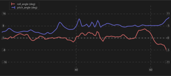

8.1.2Bode Diagram#

Estimate the transfer function of a system using the FFT of the input and output signals and plot its Bode Diagram. The first signal added to the plot will be used as input, and the second as output.

out = clab.bode(id=0, obj=None, name='')

out: Chart’s unique identifier.
idoptional: Chart’s unique identifier. This argument is used to add an object to an existing chart.
objoptional: clab.TimeSeries object.
nameoptional: Variable’s name.

Examples

chart_id1 = clab.bode()
clab.bode(id=chart_id1, obj=f['Input Signal'])
clab.bode(id=chart_id1, obj=f['Output Signal'])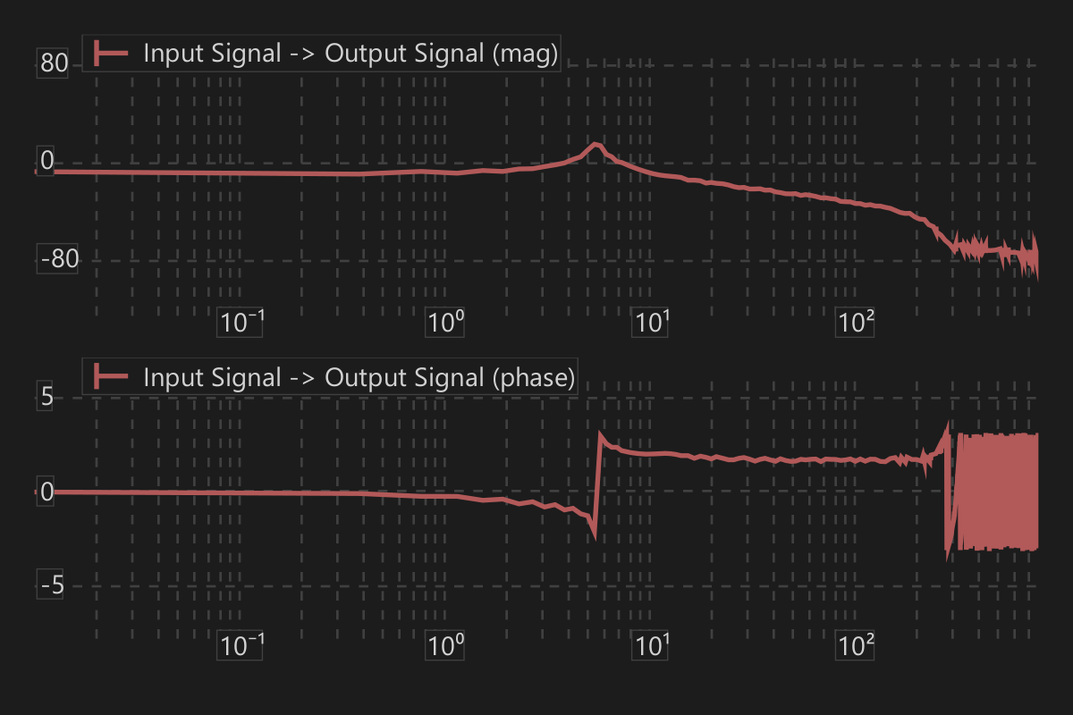

8.1.3Boolean Plot#

This function plots data points based on boolean values. A dot is plotted for each value different from zero in the data; zero values result in no plot for that specific data point.

out = clab.boolplot(id=0, obj=None, name='')

out: Chart’s unique identifier.
idoptional: Chart’s unique identifier. This argument is used to add an object to an existing chart.
objoptional: clab.TimeSeries object.
nameoptional: Variable’s name.

Examples

ts1 = clab.create_random(seed=1234, type='int', ymin=0.0, ymax=1.0, xdiff=0.5)
ts2 = clab.create_random(seed=4321, type='int', ymin=0.0, ymax=1.0, xdiff=0.5)
chart_id1 = clab.boolplot()
clab.boolplot(id=chart_id1, obj=ts1, name='VAR1')
clab.boolplot(id=chart_id1, obj=ts2, name='VAR2')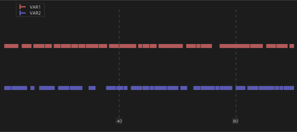

8.1.4Cross Plot#

Plot a clab.TimeSeries object against another one, displaying the engineering values in both the x-axis and y-axis.

The plotting is done by pairs: the first variable added to the chart will be the x-axis variable and the second, the y-axis. If there is an odd number of variables in the chart, the last pair will be incomplete and will not be displayed.

out = clab.crossplot(id=0, obj=None, name='', side='left')

out: Chart’s unique identifier.
idoptional: Chart’s unique identifier. This argument is used to add an object to an existing chart.
objoptional: clab.TimeSeries object.
nameoptional: Variable’s name.
sideoptional: Y-axis side. It can be either 'left' or 'right'. For the first variable, this value is ignored.

Examples

chart_id1 = clab.crossplot()
clab.crossplot(id=chart_id1, obj=f['Latitude'])
clab.crossplot(id=chart_id1, obj=f['Longitude'])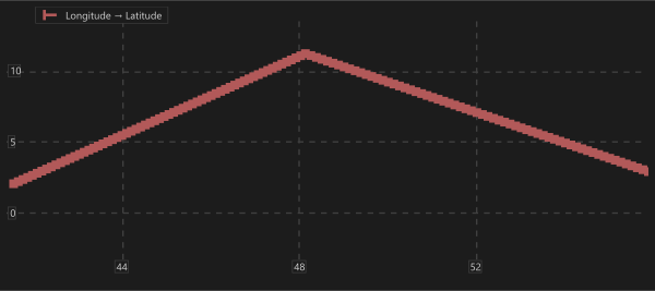

8.1.5Cross-Correlation Plot#

Calculate and plot the cross-correlation (also known as a sliding dot product or sliding inner-product) of a clab.TimeSeries object against another one (the reference variable).

The first variable added to the chart will be the reference variable.

out = clab.xcorrplot(id=0, obj=None, name='', side='left')

out: Chart’s unique identifier.
idoptional: Chart’s unique identifier. This argument is used to add an object to an existing chart.
objoptional: clab.TimeSeries object.
nameoptional: Variable’s name.
sideoptional: Y-axis side. It can be either 'left' or 'right'. For the first variable, this value is ignored.

Examples

chart_id1 = clab.xcorrplot()
clab.xcorrplot(id=chart_id1, obj=f['X1'])
clab.xcorrplot(id=chart_id1, obj=f['X2'])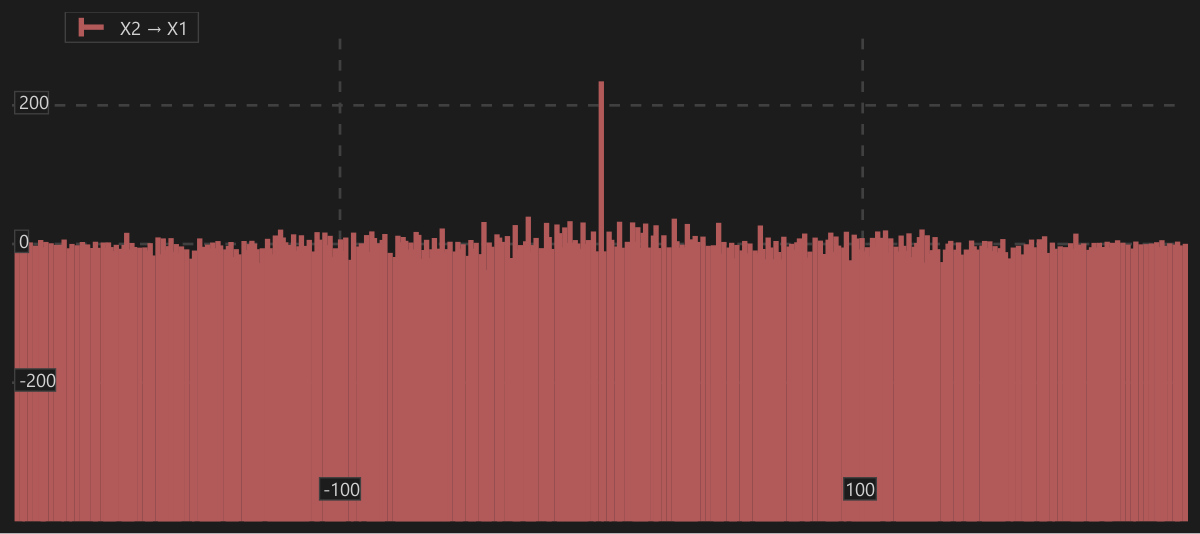

8.1.6Fast Fourier Transform Plot#

Plot the Fast Fourier Transform of a clab.TimeSeries object. The x-axis will display frequency in hertz.

If you only need the FFT data, use the clab.fftdata function (refer to Section 6.2.20).

out = clab.fft(id=0, obj=None, name='', side='left')

out: Chart’s unique identifier.
idoptional: Chart’s unique identifier. This argument is used to add an object to an existing chart.
objoptional: clab.TimeSeries object.
nameoptional: Variable’s name.
sideoptional: Y-axis side. It can be either 'left' or 'right'.

Examples

chart_id1 = clab.fft(obj=f['signal_12hz'])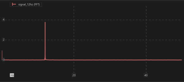

8.1.7Spectrogram Plot#

Plot the spectrogram of a clab.TimeSeries object. The y-axis will display frequency in hertz.

This function computes the Fast Fourier Transform (FFT) of consecutive time windows (spectrogram). The window size is determined by the nfft parameter, and the overlap between adjacent windows is controlled by the overlap parameter.

out = clab.spectrogram(id=0, obj=None, name='', nfft=256, overlap=0.1)

out: Chart’s unique identifier.
idoptional: Chart’s unique identifier. This argument is used to add an object to an existing chart.
objoptional: clab.TimeSeries object.
nameoptional: Variable’s name.
nfftoptional: Number of samples in the FFT window.
overlapoptional: Fraction of overlap between two windows. It can vary between 0.0 and 0.9.

Examples

var1 = clab.create_random(xdiff=0.02, dist='normal') * 0.5
var2 = clab.create_sine(xdiff=0.02, freq=16)
var3 = clab.create_chirp(xdiff=0.02)
signal = var1 + var2 + var3
clab.spectrogram(obj=signal, nfft=128)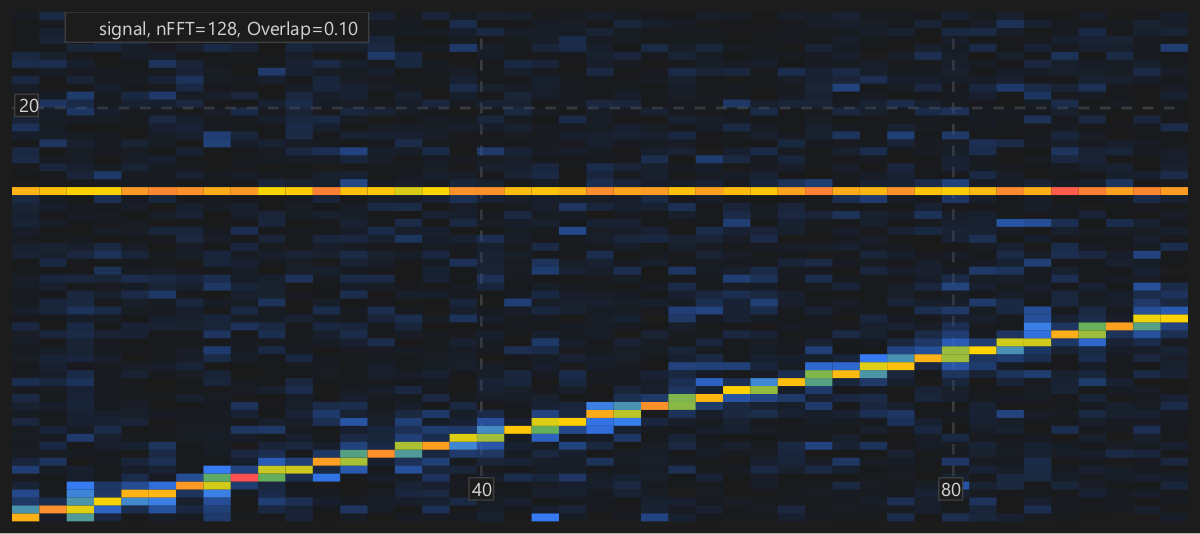

8.1.8GeoMap Plot#

Generates a geographical map visualization from latitude/longitude data contained within a clab.TimeSeries object.

Each plot supports a single variable, whose data must present the following layout:

xdata: A 1D clab.Array representing the unique longitude coordinates. The inner loop iterates through this data to determine the column position for each data point.
ydata: A 1D clab.Array representing the unique latitude coordinates. The outer loop iterates through this data to determine the row position for each data point.
zdata: A flattened 1D clab.Array representing a 2D grid of values (len(ydata) $\times$ len(xdata)). It is stored in row-major order, where all the X-values for a given Y-row are contiguous in memory. The element at a specific grid intersection is accessed using the formula: $\text{z} = x + y \times \text{len(xdata)}$

out = clab.geomap(id=0, obj=None, name='')

out: Chart’s unique identifier.
idoptional: Chart’s unique identifier. This argument is used to add an object to an existing chart.
objoptional: clab.TimeSeries object.
nameoptional: Variable’s name.

Examples

clab.geomap(obj=f['tas'])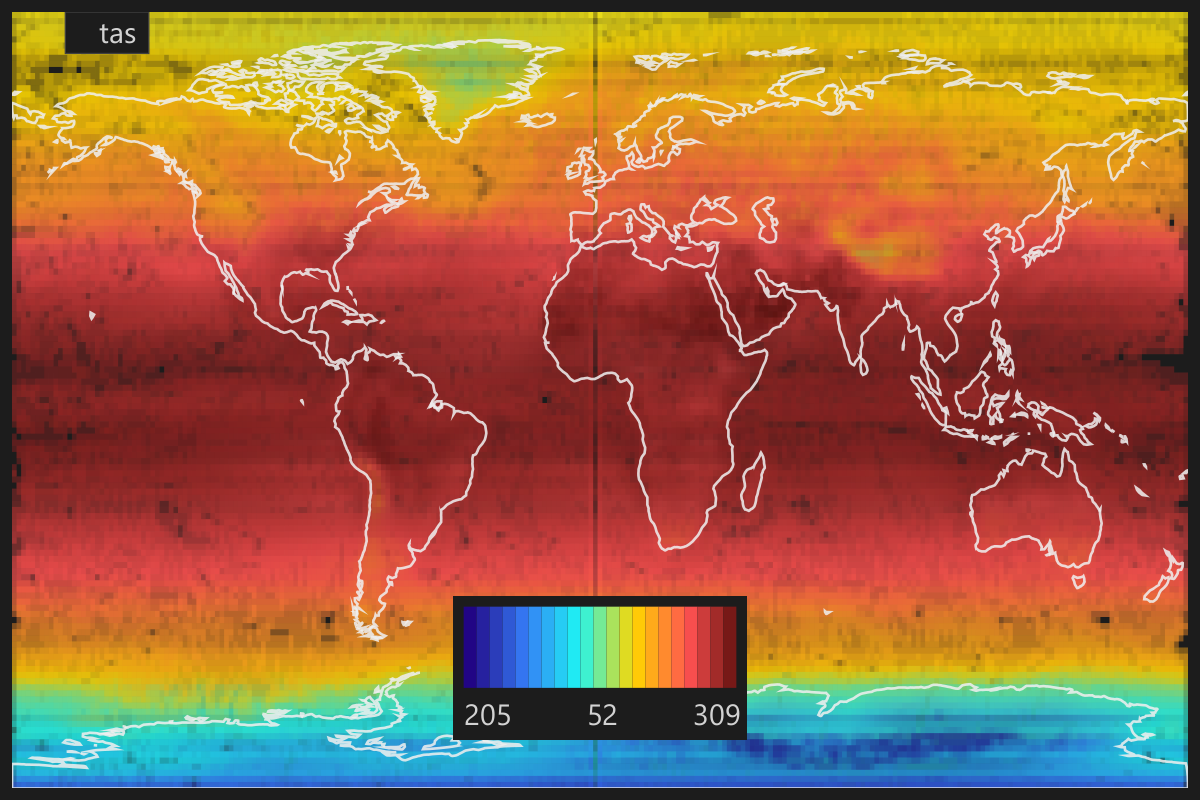

8.1.9HeatMap Plot#

Plot the heatmap between two clab.TimeSeries objects.

If you only need the underlying data matrix, use the clab.heatmapdata function (refer to Section 6.2.21).

out = clab.heatmap(id=0, obj=None, name='')

out: Chart’s unique identifier.
idoptional: Chart’s unique identifier. This argument is used to add an object to an existing chart.
objoptional: clab.TimeSeries object.
nameoptional: Variable’s name.

Examples

chart_id1 = clab.heatmap()
clab.heatmap(id=chart_id1, obj=f['X3'])
clab.heatmap(id=chart_id1, obj=f['X4'])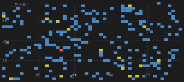

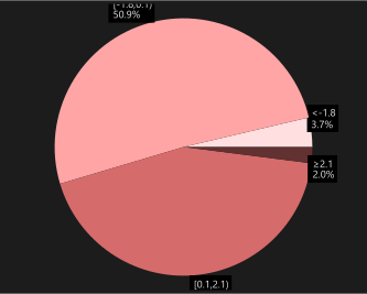
8.1.10Histogram Plot#

Plot the histogram of a clab.TimeSeries object.

If you only need the histogram data, use the clab.histdata function (refer to Section 6.2.22).

out = clab.hist(id=0, obj=None, name='', type='bar', nbins=8, bins=[])

out: Chart’s unique identifier.
idoptional: Chart’s unique identifier. This argument is used to add an object to an existing chart.
objoptional: clab.TimeSeries object.
nameoptional: Variable’s name.
typeoptional: Chart’s type. It can be either 'bar' or 'pie'.
nbinsoptional: Number of bars (for the 'bar' type) or number of slices (for the 'pie' type). Value cannot be less than 3.
binsoptional: List with the bins limits. Its length cannot be less than 2. If this argument is provided along with nbins, the latter will be ignored.

Examples

rand = clab.create_random(dist='normal')
chart_id1 = clab.hist(obj=rand, nbins=10)
chart_id2 = clab.hist(obj=rand, type='pie', nbins=4)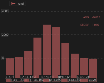

8.1.11Violin Plot#

Plot the violin diagram of a clab.TimeSeries object.

If you only need the violin data, use the clab.histdata function (refer to Section 6.2.22).

out = clab.violinplot(id=0, obj=None, name='', nbins=100)

out: Chart’s unique identifier.
idoptional: Chart’s unique identifier. This argument is used to add an object to an existing chart.
objoptional: clab.TimeSeries object.
nameoptional: Variable’s name.
nbinsoptional: Number of horizontal bars. Value cannot be less than 10.

Examples

var1 = clab.create_random(dist='normal', mean=0.0, stddev=1.0, seed=1234)
var2 = clab.create_random(dist='normal', mean=1.0, stddev=1.0, seed=1234)
chart_id = clab.violinplot()
clab.violinplot(id=chart_id, obj=var1, name='VAR1', nbins=25)
clab.violinplot(id=chart_id, obj=var2, name='VAR2', nbins=25)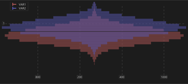

8.2Functions to Create 3D Charts#

8.2.1Time Series Plot With 3 Axes#

Plot two clab.TimeSeries objects to display engineering values on the y-axis and z-axis, with time on the x-axis. If the objects were created using built-in loaders, the x-axis will display time in seconds. Only two variables can be added to a single chart: one for the y-axis and one for the z-axis.

out = clab.plot3d(id=0, obj=None, name='')

out: Chart’s unique identifier.
idoptional: Chart’s unique identifier. This argument is used to add an object to an existing chart.
objoptional: clab.TimeSeries object.
nameoptional: Variable’s name.

Examples

chart_id1 = clab.plot3d()
clab.plot3d(id=chart_id1, name='Altitude')
clab.plot3d(id=chart_id1, name='Longitude')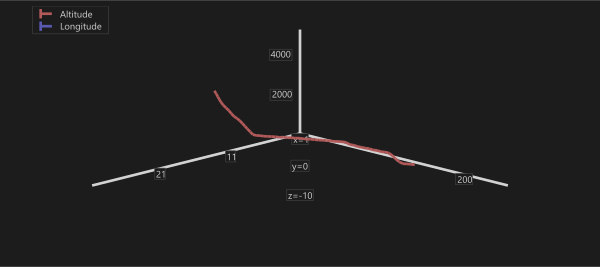

8.2.2Mesh Plot#

Plot a clab.Mesh object in a 3D surface chart.

out = clab.mesh(obj)

out: Chart’s unique identifier.
objrequired: clab.Mesh object.

Examples

mesh1 = clab.create_mesh_sinc(xdiff=1.0, zdiff=1.0)
chart_id1 = clab.mesh(mesh1)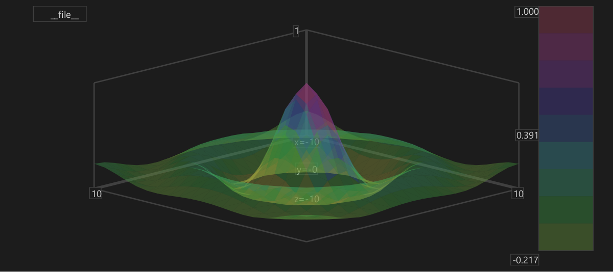

8.3Functions to Create Specialized Charts#

8.3.1Create a Synoptic Chart with Gauges#

Create a chart with gauges that visualize clab.TimeSeries values. The gauge values dynamically update based on the input clab.TimeSeries they are linked to. To update the gauge values manually, hold CTRL while moving the mouse cursor along a standard 2D chart.

out = clab.synoptic(id=0, obj=None, name='', x=-1, y=-1, width=250, min=0.0, max=10.0, red=0x36, green=0x7b, blue=0xf5)

out: Chart’s unique identifier.
idoptional: Chart’s unique identifier. Use this argument to add an object (the gauge) to an existing chart.
objoptional: The clab.TimeSeries object whose value will be displayed on the gauge.
nameoptional: The display name for the variable being visualized.
xoptional: Object’s position on the x-axis, in pixels. If this value is negative, the object will be automatically positioned in the chart.
yoptional: Object’s position on the y-axis, in pixels. If this value is negative, the object will be automatically positioned in the chart.
widthoptional: Object’s width, in pixels. If this value is negative, the object will be automatically sized.
minoptional: Minimum value in the scale (the gauge’s lower bound).
maxoptional: Maximum value in the scale (the gauge’s upper bound).
redoptional: Red channel intensity (0 to 255).
greenoptional: Green channel intensity (0 to 255).
blueoptional: Blue channel intensity (0 to 255).

Examples

chart_id1 = clab.synoptic()
clab.synoptic(id=chart_id1, name='roll_angle (deg)', min=-180.0, max=180.0)
clab.synoptic(id=chart_id1, name='pitch_angle (deg)', min=-180.0, max=180.0)
clab.synoptic(id=chart_id1, name='heading (deg)', min=0.0, max=360.0)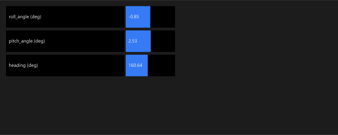

8.3.2Create a Chart with Video Frame#

Create a chart embedding a synchronized video frame from a clab.TimeSeries that contains video data. To manually scrub through video frames, hold CTRL while moving the mouse cursor along a standard 2D chart.

out = clab.video(id=0, obj=None, name='', brightness=0.0, contrast=1.0, gamma=1.0, posterization=1, thresholding=0)

out: Chart’s unique identifier.
idoptional: Chart’s unique identifier. Use this argument to add the video frame to an existing chart view.
objoptional: The clab.TimeSeries video object supplying the frames.
nameoptional: The display name or title for the video panel component.
brightnessoptional: Adjusts the overall light intensity (-1.0 to +1.0). Negative values darken the frame, while positive values uniformly brighten it. Default is 0.0 (no change).
contrastoptional: Scales the difference between light and dark areas (0.0 to 4.0). Values below 1.0 reduce contrast (flattening the image), while values above 1.0 expand it, making highlights brighter and shadows deeper. Default is 1.0.
gammaoptional: Applies non-linear gamma correction (0.0 to 99.0). Adjusting gamma optimizes the balance of mid-tones without blowing out the highlights or crushing deep blacks. Values less than 1.0 darken mid-tones; values greater than 1.0 lighten them. Default is 1.0.
posterizationoptional: Reduces the total number of color tones per channel to create a blocked, poster-like effect (1 to 128). A value of 1 retains full color depth. Higher values aggressively quantize colors, clustering gradients into flat, solid regions. Default is 1.
thresholdingoptional: Converts the image to binary black-and-white (0 to 255). A value of 0 leaves the image unchanged. Setting a value between 1 and 255 forces pixels darker than the threshold to black, and pixels brighter to pure white—ideal for segmentation or isolating high-contrast features.

Examples

clab.video(name='VideoCh1', brightness=0.5)

8.4Functions to Export Charts#

8.4.1Save Charts to File#

Save charts to file. Currently, only PDF and PNG formats are supported.

clab.save(path, id=0, size='')

pathrequired

File’s full path. The path must include the desired extension (e.g., .pdf, .png).

idoptional

Chart’s or page’s unique identifier. If not provided, all pages will be exported to the file.

sizeoptional

Page size specification. If no size is provided, the system automatically selects a default based on the file extension. Supported values are:

a3: A3 Paper Size.
a4: A4 Paper Size.
a5: A5 Paper Size.
a6: A6 Paper Size.
letter: Letter Paper Size.
<width>x<height>: Custom size specified in pixels (e.g., 200x100).

Examples

clab.save(path='c:/user/out.pdf')
clab.save(path='c:/user/out.png', id=1234, size='256x128')

8.5Functions to Modify/Configure Charts#

8.5.1Set Chart Parameters#

Set parameters for a single chart.

clab.set_chart(id, ...)

idrequired: Chart’s unique identifier.
lmaxoptional: Maximum value (in engineering units) of the left axis. Setting this parameter disables auto-zoom for the left y-axis.
lminoptional: Minimum value (in engineering units) of the left axis. Setting this parameter disables auto-zoom for the left y-axis.
rmaxoptional: Maximum value (in engineering units) of the right axis. Setting this parameter disables auto-zoom for the right y-axis.
rminoptional: Minimum value (in engineering units) of the right axis. Setting this parameter disables auto-zoom for the right y-axis.
ltickoptional: Tick step value (in engineering units) for the left axis. Setting this parameter disables auto-tick for the left y-axis.
rtickoptional: Tick step value (in engineering units) for the right axis. Setting this parameter disables auto-tick for the right y-axis.
fitoptional: Show fitted curve information. Options are 'exp', 'linear', or 'poly'.
xlabeloptional: Text to be displayed near the x-axis ticks.

Examples

clab.set_chart(id=1234, lmax=10, lmin=0)
clab.set_chart(id=1234, rtick=2.5)
clab.set_chart(id=1234, fit='linear')

8.6Functions to Create Objects on 2D Charts#

8.6.1Create a Circle#

Create a circle in a single chart.

clab.circle(chart, xcenter, ycenter, diameter, red, green, blue)

chartrequired: Chart’s unique identifier.
xcenterrequired: Circle center coordinate in the x-axis. Units match the target chart’s x-axis.
ycenterrequired: Circle center coordinate in the y-axis. Units match the target chart’s y-axis.
diameterrequired: Circle diameter. Units match the target chart’s x-axis units.
redoptional: Red channel intensity (0 to 255).
greenoptional: Green channel intensity (0 to 255).
blueoptional: Blue channel intensity (0 to 255).

Examples

clab.circle(chart=1234, xcenter=10, ycenter=20, diameter=5, red=128, green=128, blue=128)

8.6.2Create a DataTip#

Create a datatip in a single chart.

clab.datatip(chart, name, x, red, green, blue)

chartrequired: Chart’s unique identifier.
namerequired: Parameter’s name.
xrequired: Position in the x-axis (in the target chart’s coordinate units).
redoptional: Red channel intensity (0 to 255).
greenoptional: Green channel intensity (0 to 255).
blueoptional: Blue channel intensity (0 to 255).

Examples

clab.datatip(chart=1234, name='value1', x=10, red=128, green=128, blue=128)

8.6.3Create a Flag#

Create a vertical flag across all charts (if only x is provided) or a horizontal flag in a single chart (if only y is provided).

clab.flag(chart, x, y, text, red, green, blue)

chartoptional: Chart’s unique identifier.
xoptional: Position in the x-axis. If y is omitted, it creates a vertical flag.
yoptional: Position in the y-axis. If x is omitted, it creates a horizontal flag.
textoptional: Flag’s text.
redoptional: Red channel intensity (0 to 255).
greenoptional: Green channel intensity (0 to 255).
blueoptional: Blue channel intensity (0 to 255).

Examples

clab.flag(x=20.0, text='event', red=128, green=128, blue=128)
clab.flag(chart=1234, y=100.0, text='limit')

8.6.4Create Marks in All Charts#

Create marks in all charts.

clab.mark(x, width, text, red, green, blue)

xrequired: Starting position in the x-axis (in x-axis units, shared by all charts).
widthrequired: Width of the mark (in x-axis units, shared by all charts).
textoptional: Text to display on the mark.
redoptional: Red channel intensity (0 to 255).
greenoptional: Green channel intensity (0 to 255).
blueoptional: Blue channel intensity (0 to 255).

Examples

clab.mark(x=10, width=12.5, text='event', red=128, green=128, blue=128)

8.6.5Create a Rectangle#

Create a rectangle in a single chart.

clab.rectangle(chart, xcenter, ycenter, width, height, red, green, blue)

chartrequired: Chart’s unique identifier.
xcenterrequired: Rectangle center coordinate in the x-axis (in the target chart’s coordinate units).
ycenterrequired: Rectangle center coordinate in the y-axis (in the target chart’s coordinate units).
widthrequired: Rectangle width (in the target chart’s x-axis units).
heightrequired: Rectangle height (in the target chart’s y-axis units).
redoptional: Red channel intensity (0 to 255).
greenoptional: Green channel intensity (0 to 255).
blueoptional: Blue channel intensity (0 to 255).

Examples

clab.rectangle(chart=1234, xcenter=10, ycenter=20, width=5, height=5, red=128, green=128, blue=128)

8.6.6Create a Text Label#

Create a text label in a single chart.

clab.text(chart, x, y, text, red, green, blue)

chartrequired: Chart’s unique identifier.
xrequired: Text coordinate in the x-axis (in the target chart’s coordinate units).
yrequired: Text coordinate in the y-axis (in the target chart’s coordinate units).
textrequired: Text to be displayed.
redoptional: Red channel intensity (0 to 255).
greenoptional: Green channel intensity (0 to 255).
blueoptional: Blue channel intensity (0 to 255).

Examples

clab.text(chart=1234, x=10, y=20, text='this is a text', red=128, green=128, blue=128)

8.6.7Set Up Legend#

Set up a legend for a single chart.

clab.legend(chart, x, y, visible, full)

chartrequired: Chart’s unique identifier.
xoptional: Position (in pixels) on the chart for the legend.
yoptional: Position (in pixels) on the chart for the legend.
visibleoptional: If False, the legend will not be displayed.
fulloptional: If True, the legend will display full variable names.

Examples

clab.legend(chart=1234, visible=False)
clab.legend(chart=1234, x=50)

9Page Functions#

9.1Create Page#

Creates a new empty page.

out = clab.new_page(name, id=0)

out: Unique identifier of the created page.
namerequired: Page name. This value MUST be displayed in the page tab within the user interface.
idoptional: Unique identifier to assign to the page. If not provided, C-LAB MUST generate a unique identifier.

Examples

clab.new_page(id=1234, name='page 1')

9.2Delete Page#

Deletes an existing page.

clab.del_page(id=0, name='')

idoptional

Unique identifier of the page to delete.

nameoptional

Name of the page to delete.

At least one of id or name MUST be provided. If both are provided, id will take precedence.

Examples

clab.del_page(id=1234)

9.3Set Page Properties#

Modifies properties of an existing page.

clab.set_page(id, cols=-1)

idrequired

Unique identifier of the page.

colsoptional

Number of columns in the page layout. If the value is negative, the column count will not be modified.

The page identified by id MUST exist. If cols is provided and non-negative, the layout will be updated accordingly.

Examples

clab.set_page(id=1234, cols=3)

10Miscellaneous Functions#

This section defines functions for interacting with global front-end state, including charts, pages, and navigation controls.

10.1Set Global Parameters#

Sets global parameters affecting all charts and pages.

clab.set(key, args…)

keyrequired: Identifier specifying the parameter to modify.
args…required: Values assigned to the parameter identified by key. Argument types and count depend on the selected key.

'tab'

Set the active tab. Argument must be in the range 1–4.

'globaltime'

Set the current global time.

Used by time-dependent features such as clab.synoptic (see Section 8.3.1).

'timelimits'

Set the global time limits.

'timeformat'

Set the time display format used by charts. Argument must be one of the following values:

'default': Display raw time values as loaded (no formatting).
'hhmmss': Interpret values as seconds and format as HH:MM:SS (hours wrap at 24).
'unixtime': Interpret values as seconds since 00:00:00 UTC, January 1, 1970.
'gpstime': Interpret values as seconds since 00:00:00 UTC, January 5, 1980 (no leap second adjustment).

'zoom'

Equivalent to 'timelimits'.

Examples

clab.set('timeformat', 'hhmmss')
clab.set('timelimits', 10.0, 20.0)

10.2Close Charts and Pages#

Closes charts or pages by identifier.

clab.close(type, id=0)

typerequired

Identifier specifying the target to close. Valid values:

'pages': Close all pages.
'page': Close a single page.
'chart': Close a single chart.

idoptional

Unique identifier of the target. Required when type is page or chart. Ignored when type is pages.

Examples

clab.close('pages')
clab.close('chart', id=1234)

10.3Reset Parameters#

Resets global parameters affecting charts and pages.

clab.reset(key)

keyrequired

Identifier specifying the parameter to reset. Valid values:

'bookmarks': Remove all bookmarks.
'flags': Clear the cache of flags objects (see Section 8.6.3), preventing reuse in newly created charts.
'marks': Clear the cache of marks objects (see Section 8.6.4), preventing reuse in newly created charts.
'zoom': Reset zoom levels for all pages.

Examples

clab.reset('zoom')

10.4Create Bookmark#

Creates a bookmark representing a time interval in the front-end interface.

Bookmarks allow navigation between predefined time ranges and can also be created via the horizontal scrollbar context menu.

clab.bookmark(tini, tend)

tinirequired: Start time of the bookmark.
tendrequired: End time of the bookmark.

Examples

clab.bookmark(tini=1.0, tend=5.0)

11COM Server Functions#

C-LAB provides support for COM servers (IDispatch-compatible) through an out-of-process architecture. It exposes an API that allows external applications to interact with C-LAB from a separate process.

The examples in the following subsections are written in Python; however, the same principles can be applied to other programming languages.

11.1Create and Update C-LAB Objects#

11.1.1Create `clab.TimeSeries`#

Creates a clab.TimeSeries object from two arrays.

HRESULT CreateTimeSeries([in] BSTR name, [in] SAFEARRAY(VARIANT) xvalues, [in] SAFEARRAY(VARIANT) yvalues)

name: Name of the object.
xvalues: X-axis values. Must have the same length as yvalues.
yvalues: Y-axis values. Must have the same length as xvalues.

Examples

import win32com.client
obj = win32com.client.Dispatch('ClabApp.ClabObject')
obj.CreateTimeSeries('parameter1', [1,2,3,4,5,6,7,8], [10,20,30,40,50,60,70,80])

11.1.2Update `clab.TimeSeries`#

Updates a clab.TimeSeries object. If the object does not exist, it is created.

The length of an existing object is not modified:

If input arrays are shorter, remaining values are preserved.
If input arrays are longer, excess elements are ignored.

Passing an empty array leaves the corresponding data unchanged.

HRESULT UpdateTimeSeries([in] BSTR name, [in] SAFEARRAY(VARIANT) xvalues, [in] SAFEARRAY(VARIANT) yvalues)

name: Name of the object.
xvalues: X-axis values. Must match the length of yvalues or be empty.
yvalues: Y-axis values. Must match the length of xvalues or be empty.

Examples

import win32com.client
obj = win32com.client.Dispatch('ClabApp.ClabObject')
obj.UpdateTimeSeries('parameter1', [1,2,3,4,5,6,7,8], [10,20,30,40,50,60,70,80])

11.2Functions to Create 2D Charts#

11.2.1Time Series Plot#

Plots a clab.TimeSeries object. The x-axis represents time, and the y-axis represents the corresponding values. If the object was created using built-in loaders, time is expressed in seconds.

See Section 8.1.1 for the Python API equivalent.

HRESULT Plot([in] ULONGLONG chartId, [in] BSTR name, [in] BSTR side, [in] BSTR style, [out, retval] ULONGLONG* result)

chartId: Unique chart identifier. If nonzero, the object is added to the specified chart. If 0, a new chart is created.
name: Name of the object.
side: Y-axis side. Valid values: 'left', 'right'.
style: Rendering style. Valid values: 'bool', 'dots', 'line'.
result: Returns the chart identifier used for the operation. In scripting languages (e.g., Python, VBScript), this value is returned directly by the function.

Examples

import win32com.client
obj = win32com.client.Dispatch('ClabApp.ClabObject')
obj.Plot(1234, 'parameter1', 'left', 'line') # returns 1234

11.3Functions to Export Charts#

11.3.1Save Charts to File#

Exports charts to a file. Supported formats: PDF and PNG.

See Section 8.4.1 for the Python API equivalent.

HRESULT Save([in] BSTR path, [in] ULONGLONG id, [in] BSTR size)

path

Full file path, including extension.

id

Unique identifier of the chart or page. If 0, all pages are exported.

size

Output page size. Supported values:

a3: A3 paper size.
a4: A4 paper size.
a5: A5 paper size.
a6: A6 paper size.
letter: Letter paper size.
<width>x<height>: Custom size in pixels (e.g., 200x100).

Examples

import win32com.client
obj = win32com.client.Dispatch('ClabApp.ClabObject')
obj.Save('c:/file.pdf', 0, '200x100')